Why it matters?

Listening to music on YouTube has become an integral part of my life, yet a challenge persists. The music I prefer during workouts differs from my regular listening choices. However, the YouTube recommendation system fails to recognize this difference, resulting in the need to frequently switch songs between my workout sets.

To address this, I decided to create my own music classifier. By accomplishing this, I expect the distraction of changing songs diminishes, allowing me to focus more on my workout routine and utilize the time saved on song selection more effectively.

Overview

• Labeled 1300+ songs into 3 categories and collected audio feature data using Spotify API in python
• Applied feature engineering and Principal Component Analysis to create a dataset of 114 features
• Achieved f1 weighted score of 0.68 using a logistic regression model
• Created a workflow to add new songs in a sqlite3 database and update YouTube playlist automatically using Youtube API and sqlite3 database

Data Collection

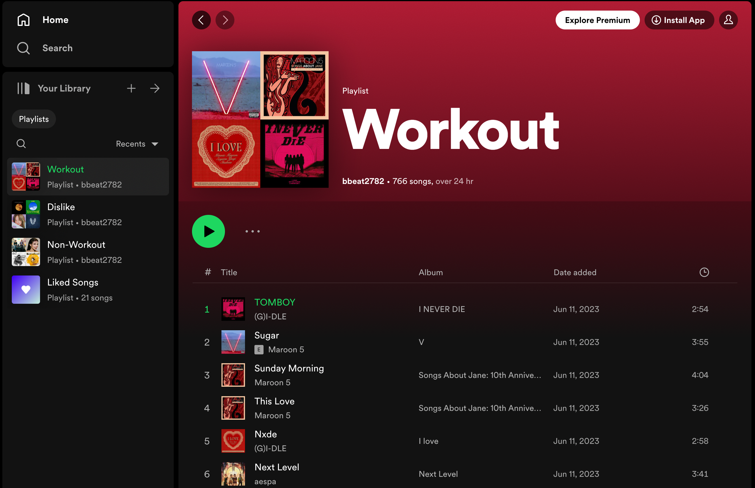
First, I labeled 1300+ songs into 3 categories on my Spotify account. The 3 categories are Workout, Non-workout, and Dislike.

Then, using the Spotify API, I collected tracks’ audio features and created a dataframe.

danceability	energy	key	loudness	mode	speechiness	acousticness	instrumentalness	liveness	valence	tempo	type	id	uri	track_href	analysis_url	duration_ms	time_signature	result
0.644	0.414	1	-6.723	1	0.0419	0.64	0	0.11	0.273	132.117	audio_features	2H1kS1ZOSTTPAFYUKjRiGo	spotify:track:2H1kS1ZOSTTPAFYUKjRiGo	https://api.spotify.com/v1/tracks/2H1kS1ZOSTTPAFYUKjRiGo	https://api.spotify.com/v1/audio-analysis/2H1kS1ZOSTTPAFYUKjRiGo	234875	4	Nonworkout
0.773	0.628	8	-5.095	1	0.145	0.0543	1.2e-05	0.0725	0.42	77.502	audio_features	3K7WdPYz7vcHMCsyBjK9vL	spotify:track:3K7WdPYz7vcHMCsyBjK9vL	https://api.spotify.com/v1/tracks/3K7WdPYz7vcHMCsyBjK9vL	https://api.spotify.com/v1/audio-analysis/3K7WdPYz7vcHMCsyBjK9vL	177653	4	Workout
0.516	0.768	9	-4.964	1	0.0362	0.00852	8.49e-06	0.136	0.204	115.005	audio_features	46bkeaB7DA45q7PdKWLFkR	spotify:track:46bkeaB7DA45q7PdKWLFkR	https://api.spotify.com/v1/tracks/46bkeaB7DA45q7PdKWLFkR	https://api.spotify.com/v1/audio-analysis/46bkeaB7DA45q7PdKWLFkR	241427	4	Workout
0.77	0.54	1	-9.087	1	0.0325	0.0347	1.49e-05	0.0326	0.804	89.989	audio_features	7yLtWtDPEC1zZpvNpbE4UA	spotify:track:7yLtWtDPEC1zZpvNpbE4UA	https://api.spotify.com/v1/tracks/7yLtWtDPEC1zZpvNpbE4UA	https://api.spotify.com/v1/audio-analysis/7yLtWtDPEC1zZpvNpbE4UA	214000	4	Workout
0.425	0.638	1	-3.184	0	0.0759	0.426	0	0.177	0.45	81.396	audio_features	3590AAEoqH50z4UmhMIY85	spotify:track:3590AAEoqH50z4UmhMIY85	https://api.spotify.com/v1/tracks/3590AAEoqH50z4UmhMIY85	https://api.spotify.com/v1/audio-analysis/3590AAEoqH50z4UmhMIY85	230667	4	Dislike

Visualizations

Imbalanced target distribution

Observations

1. Workout has the most songs, whereas dislike has the least.
   • One of the reasons is that I’m more familiar with songs I enjoy, and that led to identifying songs I dislike the least.
   • Need to take this into consideration when predicting to avoid classifying all songs into the dominant class.

Single variable distribution

Observations

1. The distinction between Workout and Nonworkout songs is apparent.
2. It’s hard to determine Dislike songs since their distribution overlap with both Workout and Nonworkout songs’ distributions.

Double variables distribution

Observations

1. The distinction between Workout and Nonworkout becomes more obvious than before.
   • Workout songs tend to have higher energy and valence than Nonworkout songs.
2. Since Dislike songs still overlap with the other two classes, I collected track’s audio analysis data and applied feature engineering to find more meaningful features.

Feature Engineering

Track’s audio analysis data has 7 keys. Those are meta, track, bars, beats, sections, segments, and tatums. Among these, I’m interested in the segments.

According to the Spotify API website, segments are divided with a roughly consistent sound. Each segment in segments contains information such as start, duration, loudness_start, loudness_max, pitches, and timbre. pitches contains an array of 12 numbers each referring to the 12 pitch classes. Their values range from 0 to 1, describing the relative dominance. timbre also contains an array of 12 numbers. But this time, each number represents different qualities of sound and is unbounded with centered at 0.

I first acquired descriptive statistics (mean, standard deviation, median, skewness, kurtosis, range, interquartile range, relative min, relative max) of loudness, pitches, and timbre from the segments. Then, after dividing a dataset into train and test sets, I calculated the means of each 12 timbre values and applied cosine similarity in relation to the target class.

The resulting data set has 331 features with 900+ rows as a training set. So to avoid the curse of dimensionality, I applied PCA for dimension reduction. I included components up to 95% of the variability and got 114 features in the end.

from sklearn.preprocessing import MinMaxScaler
from sklearn.decomposition import PCA

scaler = MinMaxScaler()
X_train_scaled = scaler.fit_transform(X_train)
X_test_scaled = scaler.fit_transform(X_test)
X_scaled = scaler.fit_transform(X)

# Include components up to 95% variability
pca = PCA(n_components=0.95)
pca.fit(X_train_scaled)

X_train_pca = pca.transform(X_train_scaled)
X_test_pca = pca.transform(X_test_scaled)
X_pca = pca.transform(X_scaled)

print(f'Num of columns after PCA: {X_train_pca.shape[1]}')

>>> Num of columns after PCA: 114

Prediction

With the dataset of 114 features, I tried using different models, including XGBoost Classifier and Support Vector Classifier. However, those models either failed to fit fast enough or were too complex for this project, which led to overfitting. Thus, I chose logistic regression, which is a simpler and faster algorithm compared to the others.

Another reason for choosing the logistic regression model is because of its precision performance in the Workout class. While the logistic regression model has a lower accuracy than the other models, it has a higher precision score for the Workout class than the other models, which is the primary goal of this project.

lr = LogisticRegression(solver='newton-cg', class_weight='balanced', max_iter=1000)
lr.fit(X_train_pca, y_train)
pred_test = lr.predict(X_test_pca)

# Calculating and printing the f1 score 
f1_test = f1_score(y_test, pred_test, average='weighted')
print('The f1 score for the testing data:', f1_test)

# Ploting the confusion matrix
confusion_matrix(y_test, pred_test)

>>> The f1 score for the testing data: 0.6816972503451451
>>> array([[15, 15, 10],
           [11, 66,  3],
           [16, 31, 98]])

The high precision score for the Workout class gave fewer misclassifications of the Workout class. According to the confusion matrix of the test data, the expected number of skipped songs when I listen to 40 songs during a workout is about 4.685 songs. $${10 + 3 \over (10+3+98)} \cdot 40 ≈ 4.685$$

To confirm this, I recorded how many songs I skip using the new classification system.

Application

Using YouTube Data API v3, I automatically update YouTube workout playlist with 40 recommended songs for my workout.

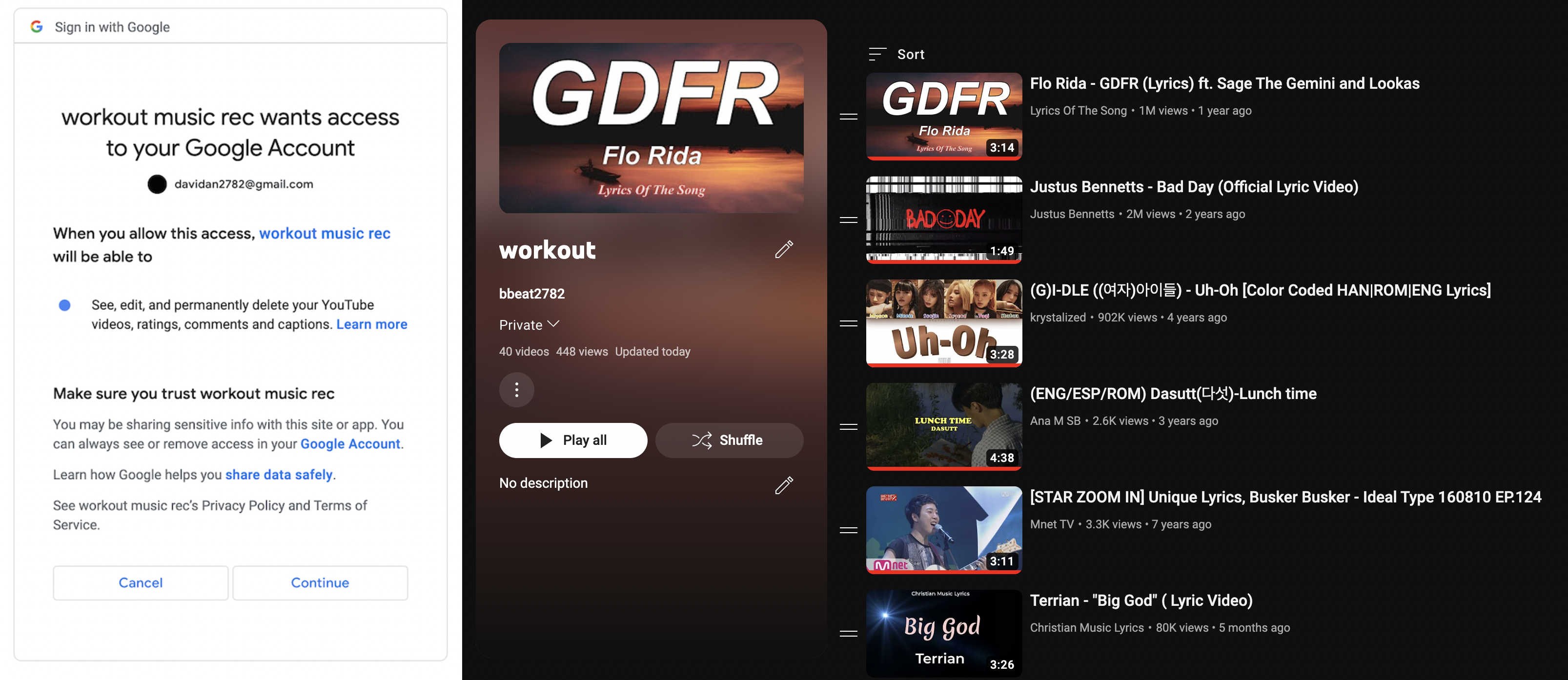
When I skip a song, I have to manually remove it from the playlist and the code will detect the skipped songs during the updating process and not recommend it in future updates.

Result

The following table is a recorded result of skipped songs during a workout with the YouTube algorithm,

day	target	songs_listened_to	skipped_songs	time_spent	exercise_time	num_songs_till_skip	skipped_songs_per_min
2023/6/11	back	33	13	30,3,18,6,10,17,19,17,24,10,35,10,13	121	2.53846	0.107438
2023/6/12	leg	24	11	30,12,3,6,6,18,6,16,6,14,17	82	2.18182	0.134146
2023/6/13	back	27	12	18,20,17,18,12,5,8,7,20,3,2,21	101	2.25	0.118812
2023/6/14	chest	29	15	16,7,20,8,20,13,10,6,9,27,9,4,6,10,4	110	1.93333	0.136364
2023/6/15	back	28	18	25,8,9,3,13,4,5,7,12,5,24,19,4,2,9,12,9,8	107	1.55556	0.168224

whereas this table contains results using the logistic regression model.

day	target	songs_listened_to	skipped_songs	exercise_time	num_songs_till_skip	skipped_songs_per_min
2023/8/19	chest	31	4	121	7.75	0.0330579
2023/8/21	back	35	6	121	5.83333	0.0495868
2023/8/22	leg	23	1	102	23	0.00980392
2023/8/23	chest	31	2	113	15.5	0.0176991
2023/8/24	back	31	1	121	31	0.00826446

As you can see in the skipped_songs columns from the two tables, my personal classification algorithm does a better job of recommending workout songs. However, comparing the raw values isn’t a good approach since the number of skipped_songs differs greatly depending on my exercise time. Thus, instead of the raw values of skipped_songs, I plotted the distributions of skipped_songs_per_min.

As you can see, the new algorithm distribution has lower skipped_songs_per_min, which means it’s doing a better job at recommending workout songs than the original method. But by how much? To compare the two distributions with a single value, I calculated the mean value of skipped_songs_per_min for each distribution.

print('Youtube algorithm: ', wo_rec['skipped_songs_per_min'].mean())

>>> Youtube algorithm:  0.10841203784175568

print('Personal algorithm: ', with_rec['skipped_songs_per_min'].mean())

>>> Personal algorithm:  0.024278991866002086

When comparing the two values, I get the following.

$${0.1084 \over 0.02428} ≈ 4.4653$$

Therefore, the new algorithm is about 4.5 times better at filtering songs I don’t listen to when I exercise.

Besides these quantitative values, I believe the workflow I built is better since it can provide more diverse playlists. When I used the YouTube algorithm, it primarily recommended songs I recently listened to. Thus, most of the time, the songs it recommended were not very much different between days, which is one of the reasons why the number of skipped songs was high. However, my personal recommendation algorithm randomly selects songs from all songs that are classified into the Workout class, and I can add any new song to the database. These two features lead to providing more diverse playlists and possibly contributed to reducing the number of skipped_songs.